Visualizing the Space of Seifert Fiberings

Introduction

One of the hallmarks of the 20^th century was the development of topology. With roots in analysis, topology is the study of geometry that does not rely on the concept of distance. For this reason, some coined the term “rubber-sheet geometry” to describe topology, as spaces in topology are considered equivalent up to arbitrary distortion. The classic example of this is the joke that a topologist can’t tell the difference between a coffee mug and a donut, since one could, in theory, distort a donut into a coffee mug.

Topology can now be used to describe a wide class of spaces, and distinguishing them in general can be somewhat challenging. For example, whilst intuitively, we know 2D space cannot be deformed into 3D space, actually proving this statement becomes surprisingly non-trivial. Now this is an example of a problem that we can at least visualize. As it turns out, start doing things like increasing dimension, or move to spaces which aren’t embeddable into 3-space, our intuition starts to run out, and we start to see the need for more formal constructions.

To tackle this problem, over the past century, mathematicians have developed various tools to transform difficult topological problems into relatively less difficult algebraic ones. One of the earliest examples of this “algebrization” process is the construction of the fundamental group for a space. The fundamental group is this idea that one could take every loop within a topological space (up to continuous deformation) and consider this collection of loops as a group (Don’t worry if you don’t know what a group is yet. We will discuss more later in the article). It turns out, however, this process really only helps classify surfaces; thus, to generalize this concept, we introduced the higher homotopy groups, which are constructed by considering all continuous maps of arbitrarily dimensioned spheres into the space in question. These homotopy groups turn out to be quite good at classifying (relatively nice) topological spaces, since if every homotopy group of two spaces is isomorphic, then the two spaces are considered homotopy equivalent (which we will discuss later). However, as it turns out, these are generally impossible to compute; even something as simple as the $n$-spheres is not fully understood, thus severely limiting their use in topology.

Herein comes homology to help save the day. Instead of discussing loops up to homotopy, we discuss loops up to homology, which is a slightly weaker (and much more difficult to explain) notion of equivalence. At the price of its distinguishing powers, it offers great computability, which in turn makes it a more useful theory. Though as it turns out, the task of classifying all spaces up to homotopy is unsolvable, rendering the search for a theory that offers both great computability and a strong equivalence a futile effort.

However, while these tools offer valuable analytical insight into such spaces, they often fall short in cultivating an intuitive grasp of these topological concepts. Although relying too heavily on visual intuition for abstract geometric concepts can be misleading, dismissing it entirely would be a mistake. Visual intuition can be immensely helpful in developing an understanding of complex geometric ideas and pushing the boundaries of our knowledge. Moreover, visual representations also serve as powerful tools for inspiring the next generation of mathematicians and conveying the true spirit of mathematical thinking.

Basic Constructions

Since this article is mostly targeted towards people with little math experience, there are some constructions important to our discussion that we’d like to go over. For readers who are already familiar with algebraic topology, this section can be skipped without any loss of continuity.

Topology

As mentioned before, topology is a generalization of geometric spaces by removing the mention of distance. We will begin our investigation of topological spaces by understanding how we can generalize geometry and the notion of space to a metric space. A metric space is a set together with a metric, defined as some function satisfying a set of properties. The actual definition here is not important, but I include it below:

A metric space is an ordered pair $(X,d)$, where $X$ is some set and a metric $d:X \times X \to \real_{\ge 0}$, such that the following are true:

1. For any $x\in X$, $d(x,x) = 0$,
2. (Positivity) For any $x,y\in X$ such that $x\neq y$, $d(x,y)\neq 0$
3. (Triangle Inequality) For any $x,y,z \in X$, we have $d(x,y)+d(y,z) \ge d(x,z)$

If the name hadn’t already given it away, the following axioms suggest that a metric is the generalization of a distance function.The first two properties are relatively easy to interpret. The triangle inequality suggests that in a metric space, the shortest path between two points is just a straight line between them. Then, on a metric space, we can understand the notion of limits and continuity by considering open balls in $X$ by considering all subsets of the form \(B(x_0,r):=\{x\in X \mid d(x,x_0) \lt r\}.\) For those familiar with the definitions of limits and continuity on the real line, we can rewrite that definition with the concept of open balls on the real line, which are just open intervals. We can then expand the definition of an open ball to a general notion of an open set by considering all subsets of $X$ that are arbitrary unions of open balls.

But since these open balls are just specific subsets of the entire space, if we just consider these balls as sets indexed by a point in $X$ and some positive real number, the fact that these arise from some metric is irrelevant when considering the question of continuity. For this reason, we can define a more general concept of topology by considering only the collection of subsets satisfying some properties, which we call basic open sets. Then by forming the arbitrary union of these basic open sets, we obtain a topology. Of course, we can also skip this step of forming basic open steps and define an open set to start. With everything we’ve talked about, we finally arrive at the modern definition of a topological space; however, a full understanding is not necessary for further discussion.

A topological space is an ordered pair $(X, T)$, for $X$ is a set and $T\subseteq P(X)$ called the collection of open sets, satisfying the following properties:

1. $\varnothing, X$ are open sets,
2. Arbitrary unions (possibly infinite) of open sets are open sets,
3. Finite intersection of open sets is open.

For those interested, of course, one could check that our definition of open sets on a metric space indeed satisfies the axioms to form a topological space. Although before, we defined continuity with respect to basic open sets, we can equivalently define continuity using open sets. This is often seen as the preferred method of defining continuity on any topological space.There are many reasons why thinking about topology with respect to open sets is more useful than thinking about topology with respect to basic open sets. For instance, the collection of open sets remaining closed under arbitrary union is incredibly powerful when it comes to manipulating these sets in proofs. However, more importantly, the collection of open sets can be understood as the collection of sets without a boundary (for sufficiently nice spaces). Since closed sets in topology are defined to be the complement of an open set, they can in turn be interpreted as sets with boundary.

In topology, we will only consider continuous maps, and in particular, when a map is continuous and a bijection, if the inverse of this map is continuous, then we say this map is a homeomorphism.Note that there exist continuous bijections with discontinuous inverses. When there is a homeomorphism between two spaces, we say they are homeomorphic, which is to say these topological spaces are essentially equivalent (up to a relabeling of the points).

A slightly weaker notion of equivalence that is often useful is homotopy. In particular, we are interested in the notion of homotopic functions. Two functions are considered homotopic when there exists a continuous deformation between them. Formally, we give the following definition:

Two continuous functions $f_0,f_1: X \to Y$ are homotopic when there exists a continuous function $H:X \times [0,1] \to Y$ such that $H(x,0)=f_0(x)$ and $H(x,1)=f_1(x)$.

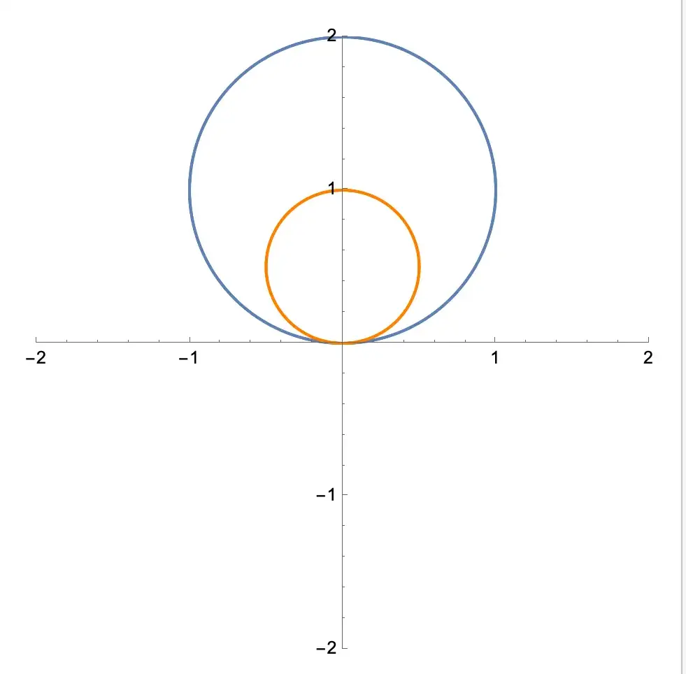
An interesting case is continuous functions of the form $f:S^1 \to X$, or loops in $X$.We often require loop homotopies to preserve basepoints, which our visualizations here show. We can visualize the deformation in the following image:

The next image is an example of loops that aren’t homotopic.

We can also define a slightly weaker notion of equivalence on spaces, namely homotopy equivalence. Two spaces are homotopy equivalent when there’s some continuous deformation between them. Formally, we require

Two topological spaces $X$ and $Y$ are homotopy equvilent iff there exists $f:X \to Y$ and $g:Y \to X$ such that $f\circ g$ and $g\circ f$ are homotopic to the identity.

For example, a point and a disk are evidently not homemorphic, since their underlying sets have different cardinality. They are, in fact, homotopy equivalent, as one can crush a disk to a point continuously. However, a circle is not homotopy equivalent to a point since no matter how much one deforms a circle, it will always have a “hole” in the middle.

Manifolds

A topological space is an incredibly powerful definition, which is often too broad for application in geometry. Thus, we often restrict ourselves to a more selective class of well-behaved topological spaces known as manifolds. Put simply, a manifold is a topological space that is locally Euclidean at every point. Thus just means that at any point, we can find some open set around it (or a neighborhood) that is homeomorphic to Euclidean space.

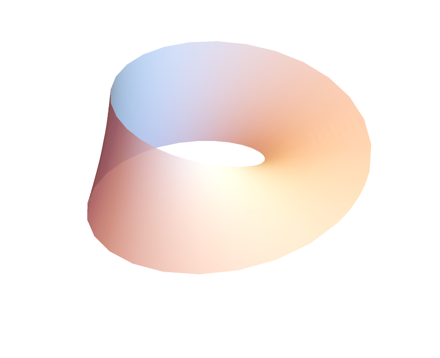
Many common examples of topological spaces indeed admit manifold structures. Take, for example, the normal sphere. For any point, if we take a sufficiently small disk around it, then deform it in a way to remove the curvature, we find that this set is homeomorphic to any open disk in the plane. Since any open disk in the plane is homeomorphic to the entire plane, the open disk we took from the sphere is also, in fact, homeomorphic to the entire plane. For this reason, the sphere is a manifold. Other common examples of manifolds are shown below.Technically, the Möbius strip is a manifold with boundary since any neighborhood of a boundary point is homeomorphic to the half plane. We will not fuss with the technicals in this article, thus we will ignore this technicality.

In the subsequent section, we will go into more details of examples of manifolds that we are interested in, but for those who want a better understanding of a manifold, below, I have left the rigorous definition of a smooth manifold, although a full understanding of this definition is not necessary for the remainder of this article.

Let $M$ be a topological. $M$ is a smooth n-manifold structure if for a collection of homomorphisms $\{\phi_\alpha: U_\alpha \to W_\alpha\}_{\alpha\in I}$, the following hold:

1. $\{U_\alpha\}_{\alpha \in I}$ is an open cover of $M$,
2. $W_\alpha$ are each subsets of $\real^n$,
3. For each $U_\alpha \cap U_\beta \neq \varnothing$, the composition $\phi_\alpha \circ {\phi_\beta}^{-1}\mid_{\phi_\beta(U_\alpha \cap U_\beta)}$ is smooth (infinitely differentiable).

The last condition only needs to hold if we want our manifold structure to be smooth. By removing it, we would obtain a more general manifold known as a topological manifold. Of course, in the case of smooth manifolds, we’d ike our functions to preserve this smooth structure, which is where smooth maps come in. A map $f:M \to N$ between smooth manifolds is smooth if and only if for any $\alpha,\beta \in I$, the composition $\phi_\alpha \circ f \circ {\phi_\beta}^{-1}\mid_{\phi(U_\alpha \cap U_\beta)}$ is smooth in $\real^n$. If a map is a bijection with a smooth inverse, we say this map is a diffeomorphism, and similarly, if there exists a diffeomorphism between two spaces, these spaces are said to be diffeomorphic.

Important Examples of Manifolds

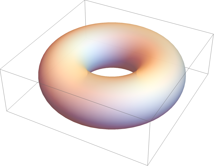
Like Euclidean space, we can also take the Cartesian product of spheres. For instance, the torus can be represented by $S^1 \times S^1$ as seen in the image below.

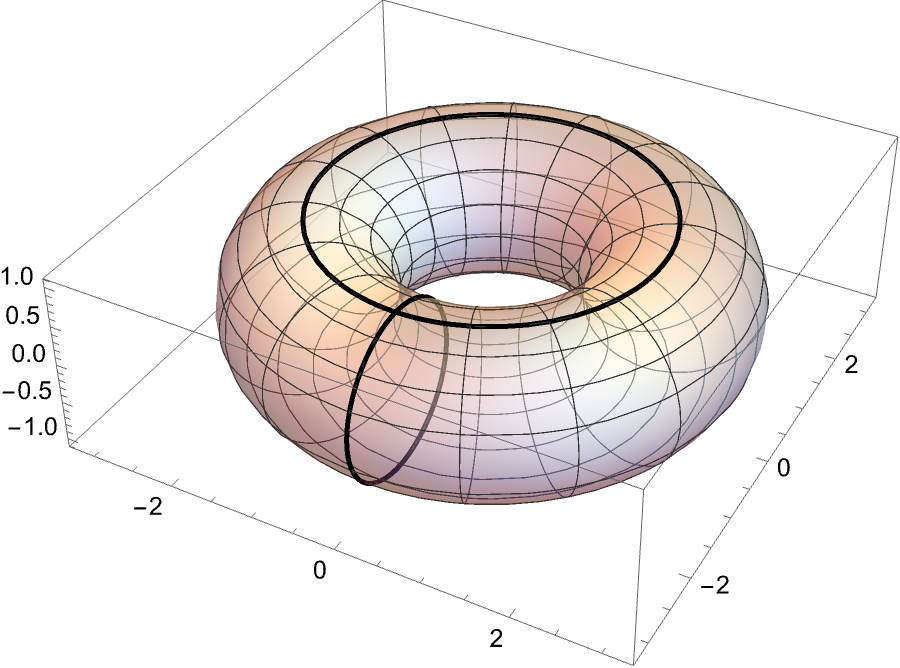
If we sit and ponder this for a minute, we should be able to see that we can identify each point as an ordered pair in the form $(t,s)$, where $t$ and $s$ range from $0$ to $2\pi$ representing points on the longitudinal and meridian circles, respectively.

Taking some inspiration from this construction of the torus, let’s construct $S^2\times S^1$ in the following way: Start with a solid ball with a cavity at the center. Then we can see that each point can be completely identified by $(t,s)$, where $t$ is a point on the inner sphere and $s$ is the distance from the origin. Effectively, what we have here is $S^2 \times I,$ where $I$ is the interval between the two spheres. Then, if we identify the two points where the ray from the origin intersects the two spheres, we get $S^2 \times S^1$. It may seem immediately obvious that this manifold is not embeddable into 3-space, thus making it impossible to visualize (at least intuitively). Thus, to make sense of this, we have to imagine each boundary sphere is a portal sending a point to the inner sphere from the outer sphere or vice versa. To harbor a deeper understanding, we visualize a loop in $S^2 \times S^1$ by our representation of the space in the image below:

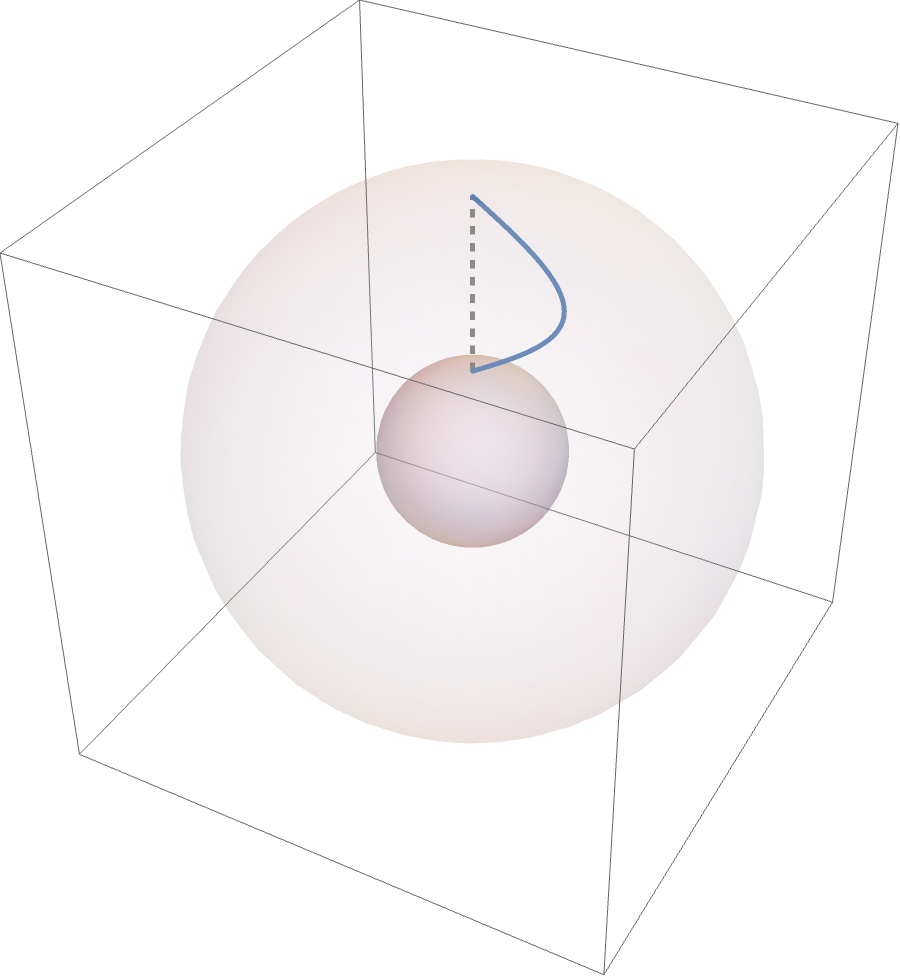
Notice that at the points where this loop crosses the boundary must lie on the same ray. If this didn’t happen, the immediate consequence would be that this loop is not continuous.

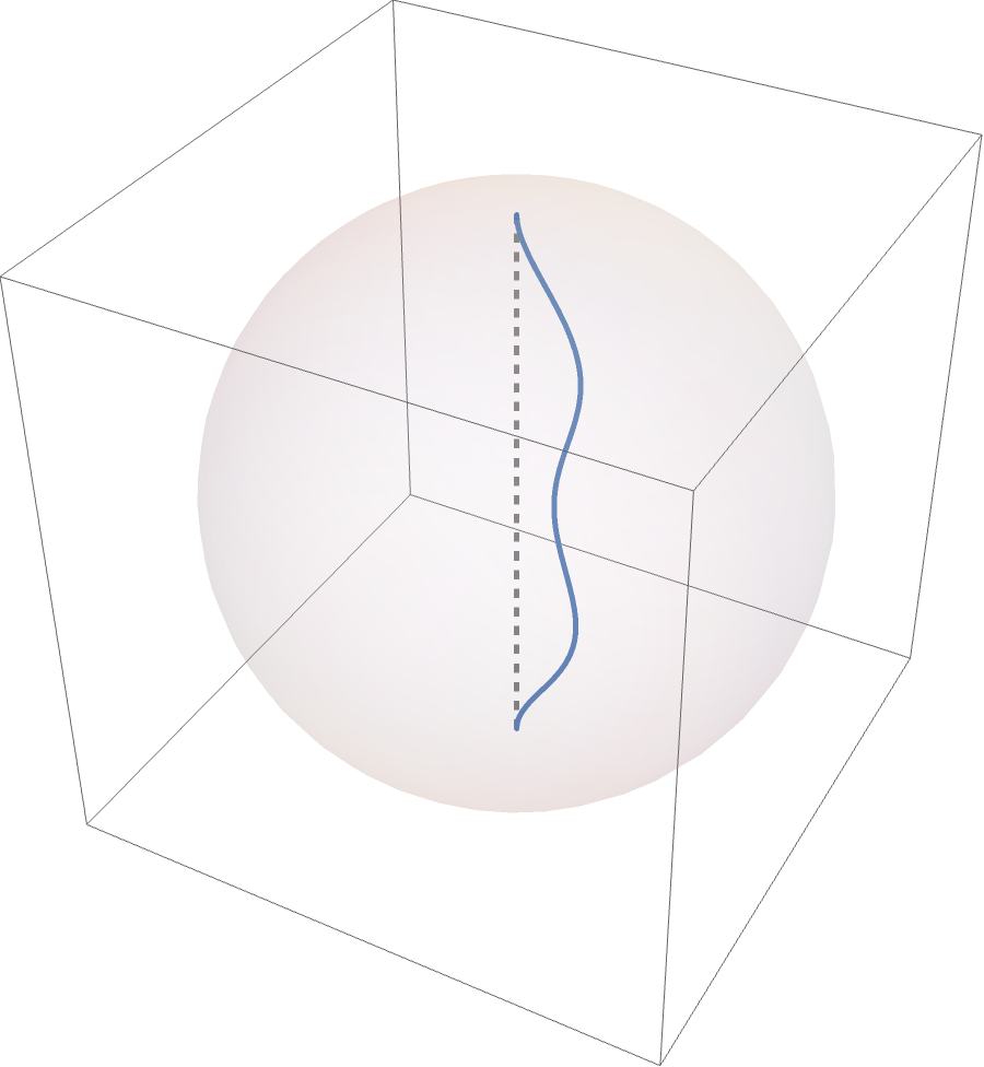
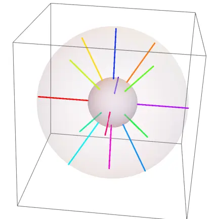
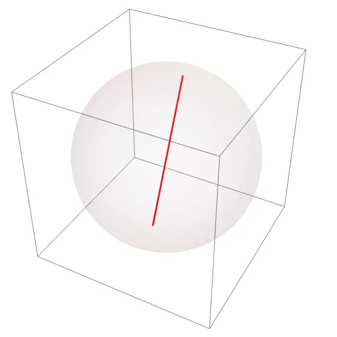
We will now move on to discussing $\rp^3$. Similar to before, $\rp^3$ isn’t embeddable into 3-space, hence we need to come up with an alternative way to think about it. This time, we will start with $D^3$, and instead, we will identify the antipodal points on the boundary. Similar to before, to conceptualize, we imagine the boundary as a portal sending points on the boundary to a point on the boundary on the opposite side of the sphere. A loop in $\rp^3$ in this presentation can be seen in the following image:

For those familiar with the quotient topology, we can give the following definition:

Let $f:\partial D^3 \to \partial D^3$ be the antipodal map (i.e. $f(x)=-x$). Then \(\rp^3:= D/\sim,\) where $x\sim y$ iff $y$ is the image of $x$ under $f$.

One could easily check that $\sim$ is an equivalent relation and definition agrees with our visual definition of $\rp^3$.

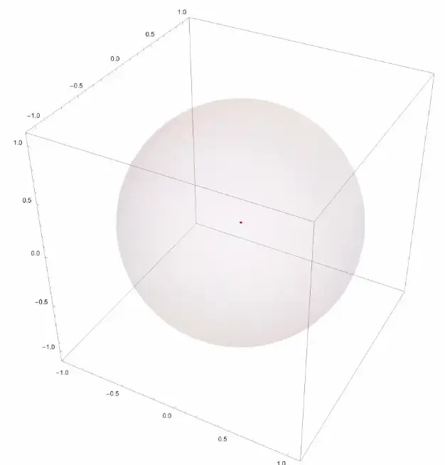
The important fact about $\rp^3$ is that it is diffeomorphic to $SO(3)$.The set of special orthogonal matrices, or just rotation matrices in 3-dimensional real vector space To show this informally, let’s consider a point in $\rp^3$. To identify an element in $SO(3)$ with a point in $\rp^3$, we start by identifying the axis of rotation.The axis of rotation must exist as a consequence of basic linear algebra. For any $3\times 3$ matrix, to find the eigenvalues, we have to solve a degree-three polynomial. Since such a polynomial must have one real solution, any $3\times 3$ matrix must have one real eigenvalue. Thus, it remains to prove that if a matrix has determinant one, this eigenvalue must be one. Then, if we map this axis to a line going through the origin of our representation of $\rp^3$, then we can determine a unique point on this line by the amount and direction of rotation. Evidently, the center of presentation of $\rp^3$ represents the identity matrix in $SO(3)$, and the point in this image

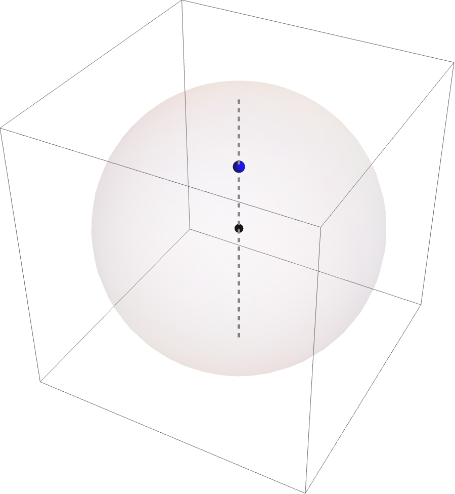
is a $90^\circ$ rotation around the $z$-axis counter-clockwise (depending on choice of orientation), if we assume the point is exactly halfway to the boundary.

Groups

Groups have become one of the most essential concepts in all of modern algebra. Now, with most things in mathematics, I could just opt to give the definition of a group, and whilst the definition is not too difficult to understand, at first glance, the motivation behind this construction may be difficult to see. However, the good news is that groups occur rather naturally in our world in more ways than one may expect.

As with all things mathematical, group theory got its start from the study of one simple concept: The action. To understand this, let’s consider the following setup of a town.

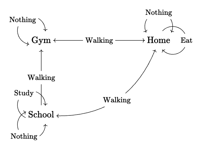
In our town, represented by the vertices on the graph, we have a house, a gym, and a school. Between the vertices, I’ve included some arrows that indicate the actions that someone in this town can take at each given location. Since at a given location, we can always choose to do nothing, at each location, we have the identity self-loop. The double arrows represent actions that are invertible, hence if you take an action, then its inverse, it’s the same as just taking the identity action. Since, for example, the action of eating is not invertible (unless you can throw up on command), it is represented by a single arrow. The act of walking to school from home is invertible since you can always just walk back home.The act of walking to the gym from school shall be left uninvertible since the school disallows smelly students from entering the premises. The first thing we should notice is that the set of possible actions someone can take in this situation is fully dependent on the location, or the vertices, and that by combining any two actions, we can combine to form a new action. Hence, we can assign a new symbol to the composition of eating at home, then walking to school. Symbolically, we can represent this composition of actions as a sort of multiplication, and we notice immediately, this multiplication is associative, namely, for three actions represented by $a, b, c$, we have \(a \cdot (b \cdot c) = (a\cdot b) \cdot c.\) What we’ve described here is essentially a category , and whilst this structure has many deeper implications in math, for our purposes, we will be interested in categories solely as a pitstop before defining a group.

Now, for our purposes, a category is still too broad a definition; hence, to make the underlying math more interesting, we shall require every action to be invertible, hence for every action there exists an inverse action whose composition (in both directions) is the identity action. With this requirement of inevitable actions, what we have now is known as a groupoid. Now, at this point, let’s take a step back from the town analogy and apply this new groupoid structure to a topological space.

We shall define a path in a topological space $X$ as a continuous map $f:[0,1] \to X$. Let $\Pi_1(X)$ be the set of all these paths in $X$ up to homotopy (preserving endpoints). Then, to put a groupoid structure on this, interpret each of these paths as the action of moving from $f(0)$ to $f(1)$ in $X$. Immediately, we notice that each action in $\Pi_1(X)$ is invertible by just reversing the direction of parameterization, and that the identity action is just the constant path. With a bit more work, one could also check that path concatenation is indeed associative. Like before, we can give this groupoid a visual representation as a graph, where the vertices are individual points in $X$, and the edges between vertices are paths between points. What we’ve described here is what’s known as the fundamental groupoid.

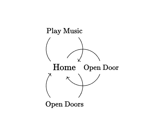
Now the groupoid is a wonderfully interesting structure, but still a bit too broad for many applications. Hence, to simplify, we normally consider groupoids with a single vertex; hence, all the actions become self-loops on this single vertex. This is what we call a group. We can similarly define the fundamental group $\pi_1(X,x_0)$ by restricting our attention to one base point, $x_0$, in $X$; hence, every action in $\pi_1(X,x_0)$ is a loop (up to homotopy) containing $x_0$. In our town analogy, this would correspond to only considering actions which are invertible and location preserving; hence, the following diagram:

Now, like before, for those who are interested, we have the formal definition of a group as seen in any algebra textbook:

Let $G$ be a set and $\cdot: G \times G \to G$ be a map such that the following are true:

1. (Identity) There exists $e$ such that for every $g\in G$, $g\cdot e = e \cdot g = g$.
2. (Inverse) For every $g\in G$, there exists $g^{-1}$ such that $g\cdot g^{-1} = g^{-1}\cdot g = e$
3. (Associativity) For every $g_1,g_2,g_3 \in G$, $g_1 \cdot (g_2 \cdot g_3) = (g_1 \cdot g_2) \cdot g_3$.

Homology

One of the biggest issues with the fundamental group as described above is that it’s really only good for distinguishing surfaces or lines. Where this theory starts to fail is when we try to use it to classify higher-dimensional spaces. For this reason, a theory was developed where we consider all maps of the form $f:S^n \to X$ (up to homotopy) containing some base point for some space $X$. These groups are known as the higher homotopy groups, and they generalize the fundamental group to higher-dimensional spaces, but this added complexity makes it difficult to compute, which hinders its usefulness.

Homology solves many of these issues; however, the exact motivation of the modern definition is much trickier to trace. Here, we will give a brief overview of the key points. The study of homology originated from Riemann and his study of line integrals of the form \(\int_C X\,dx + Y \, dy\) where $C$ is some collection of simply closed curves, on various surfaces. If $\pdiff{X}{y} - \pdiff{Y}{x}=0$, Stokes’ theorem reveals that this integral vanishes for any $(X,Y)$ if and only if $C$ forms a complete boundary of some region in the surface.To make the following rigorous, one would have to fuss with orientation. However, since we are not looking for rigor, we will ignore such complications and only use examples where this is a non-issue. Then he considered sets of simply closed curves for which the integral doesn’t vanish for any subset and is maximal with respect to this property. He noticed the size of these sets was independent of the choice of curves. Then he defined an $(n+1)$-fold connected manifold as a manifold where these sets contain $n$ curves.

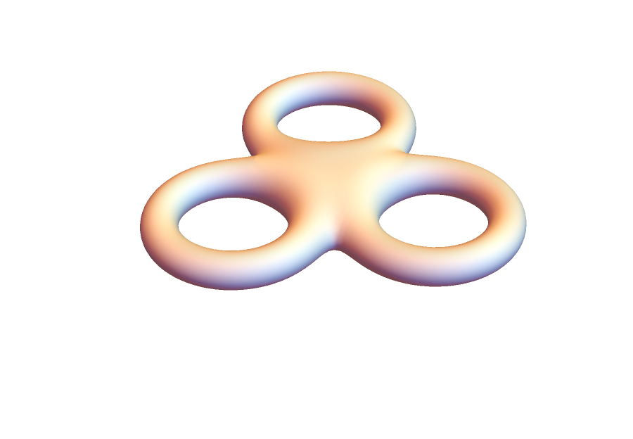
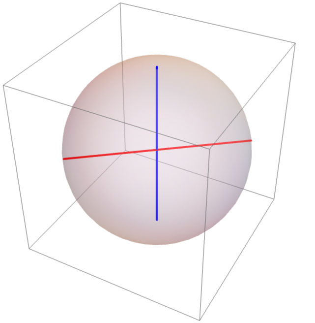
By this definition, we observe that an annulus is $2$-fold connected, a with some careful consideration, a torus is $3$-fold connected as indicated by the figures below.

Intuitively, this primitive version of homology measures how close a space is to being $1-fold connected$ or simply connected.This just means that a space is homotopy equivalent to a point In addition, Riemann noticed that this number is invariant under homotopy equivalence.

This idea of identifying curves that form a complete boundary can be generalized to higher dimensions; however, this would take many decades, which we will gloss over. It also turns out this presentation of homology had many flaws (in particular in its way it interacted with non-orientable surfaces like the Möbius strip). Only until the end of the 19th century would a modern form of homology take shape in the hands of Poincaré. This definition also led Poincaré to the identification of the now familiar torsion elements, which we will not get into. To make everything clear, the term cycles was coined to refer to the generalized simply closed curves as Riemann had been considering; cycles which formed a complete boundary became known as boundaries. It wasn’t until 1925 that Noether gave homology the group interpretation that it sees today.

However, even with its many flaws, one can still use this to understand a few things. In particular, it gives an intuitive understanding of the homologous generators. It turns out these maximal sets form a basis for $H_1(X)$, or the first homology group of a given space $X$.More precisely, these sets are a basis for the $\integ/2$ vector space $H_1(X;\integ/2)$. This can be quickly corroborated by the fact that \(H_1(A)=\integ, \quad H_1(S^1 \times S^1) = \integ \times \integ\) where we take $A$ is anulus. These sets generate the first homology group since they are curves (hence 1D objects). We can generalize this to further dimensions by considering cycles of higher dimension; however, this is where we will end our discussion to avoid getting too technical.

Seifert Fiberings

While a Seifert fibering is a general construction that can exist on a wide class of manifolds, for our discussion, we will restrict our discussion to only consist of a specific class of Seifert fiberings on $S^2 \times S^1$.

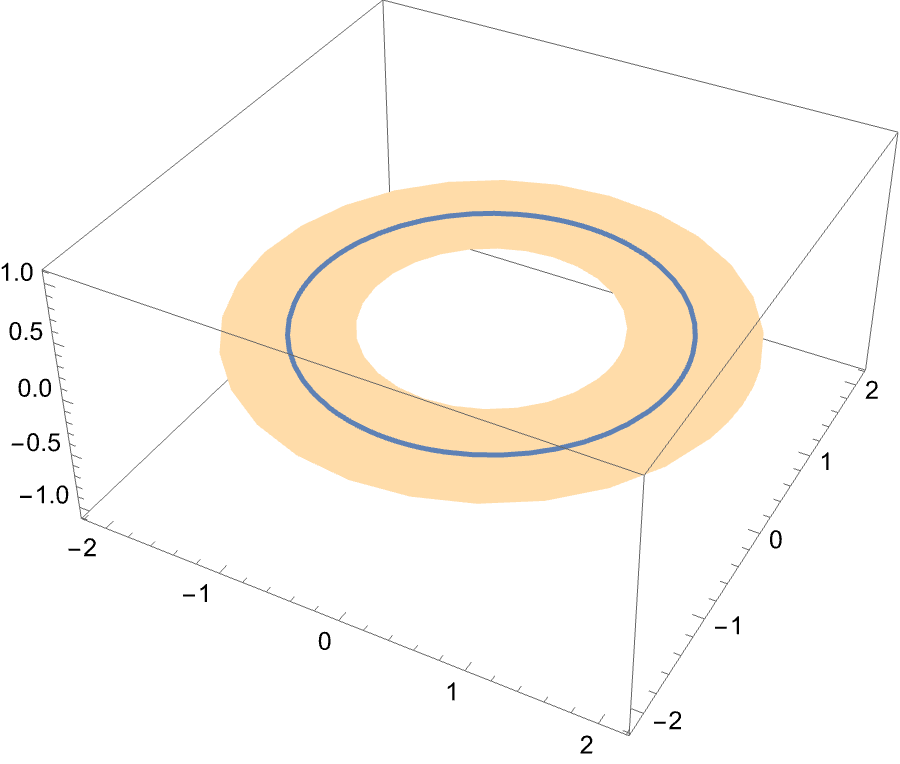
Let’s first talk about a fiber bundle. Loosely speaking, a fiber bundle is a way to break down a total space into individual fibers attached to some base space. For example, we can consider an annulus as a collection of fibers stemming from the inner circle stretching outwards, like in the following image (of course, we have only selected a finite number of fibers to display).

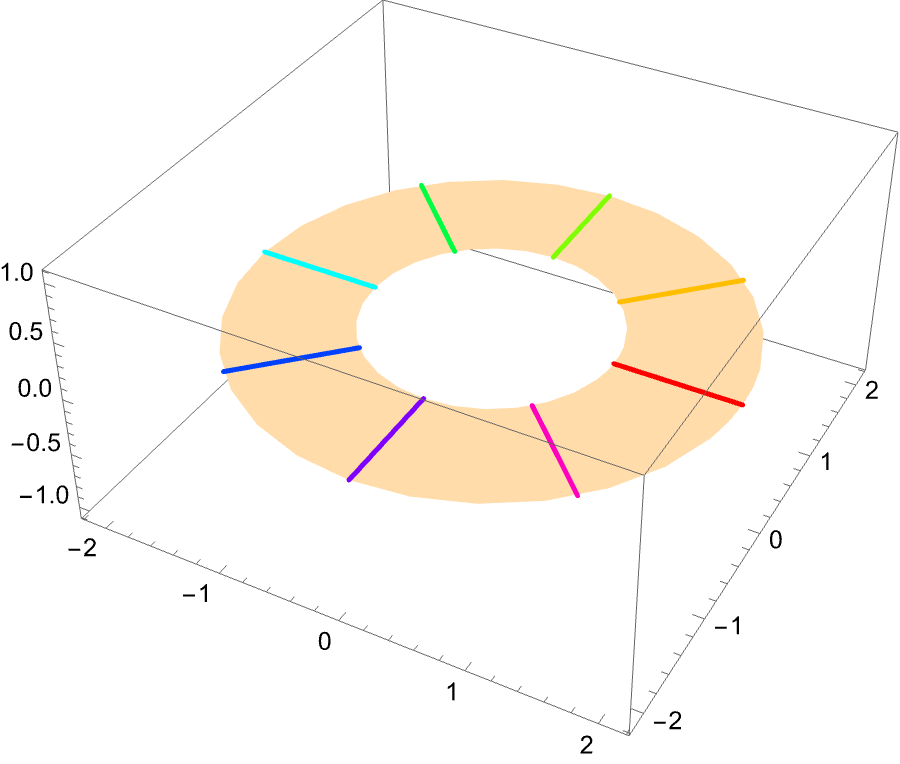
Thus, we can consider the annulus as a fibering of $S^1$ by line segments. To make sure our fiber bundles are well behaved, we often require that our bundles are locally trivial, which just means our bundle has a neighborhood around each point that looks like the cartesian product of the neighborhood and the fiber.

We can give a formal definition of what we explained here, and it goes as follows:

A fiber bundle over some space $B$ and fiber $F$ is a map $p:E \to B$ such that

1. for each $x \in B$, $p^{-1}(x)$ is homeomorphic to $F$.
2. (local triviality) for some open $U\subseteq B$ such that $p^{-1}(U)$ is homeomorphic to $U\times F$ by some basepoint preserving homemomorphism.

Additionally, we denote $E$ as the total space.For those of you who have studied algebraic topology, this definition may resemble the definition for a covering space. It turns out these things are somewhat related in the sense they both satisfy a homotopy lifting property.

It should be noted here that fiber bundles are not generally unique, and any triple consisting of a base space, a total space, and a standard fiber can give rise to an enormous set of fiberings, which is what our proceeding sections will address.

Now, for our purposes, we will consider a fiber structure on $S^2\times S^1$, where each individual fiber is homeomorphic to $S^1$ (i.e, non-self-intersecting loops). As such, an example of such a fibering would be what’s known as the trivial Seifert fibering of $S^2 \times S^1$ and is displayed below.

We will use the symbol $T$ to denote this specific fibering. In this article, we will study all such fiberings isomorphic to this trivial fibering, and we consider two fiberings to be isomorphic iff there exists some basepoint preserving diffeomorphism from $S^2 \times S^1$ to itself. We can collect all of these fiberings and put them into a set called $\sym{SF}(S^2\times S^1, T)$ and put a topology on it. We won’t go too much into detail about how this is done, but loosely speaking, we can quantify closeness between two fiberings by observing how big a transformation we need to perform to get from one to another.

For any space $X$, if we let $\Omega X$ represent the space of loops arising from sme fixed basepoint, we have the following theorem as shown in [WY24]:

The space $SF(S^2\times S^1,T)$ is homotopy equivalent to $\Omega SO(3)$, which is homeomorphic to $\Omega \rp^3$. Since $\Omega \rp^3$ has two path components, each homeomorphic to $\Omega S^3$. Thus, we have for each path componentIt suffices to consider the homology in each path component separately, since the disconnected path components don’t really interact with each other. If we insist, we take the homology of the entire space by simply taking the direct sum of the homology groups in each dimension. \(H_n(\Omega S^3) = \begin{cases} \integ &\text{if } n \text{ is even};\\ 0 &\text{if } n \text{ is odd} \end{cases}\)

We won’t go into the details of proving this theorem, but we will tackle one small detail: how do we know $\Omega\rp^3$ has two path components.

Recall, a space is path-connected if between every two points in the space, there exists some path. In the context of loop spaces, paths between two loops are essentially homotopies between them (i.e., functions that deform one loop to another). In $\rp^3$, there are always two homotopy classes of loops, evident by observing $\pi_1(\rp^3)\simeq \integ/2$.

However, let’s try to demonstrate this fact visually. Below, I have included some animations of loops in $\rp^3$ deforming. What I want you to pay attention to is the number of times a loop intersects the boundary.

In the animation below,

we see a loop expand from the constant loop centered at the origin to larger and larger loops. If we pay attention to the number of intersections with the boundary (assuming this loop is not tangent to the boundary anywhere), this number is always divisible by 4. It turns out the divisibility of the number of intersections forms a sort of homotopy invariant: No matter how you deform the constant loop, this number will always be divisible by 4. We will denote these as the trivial loops in $\rp^3$.

Then, examine this next animation

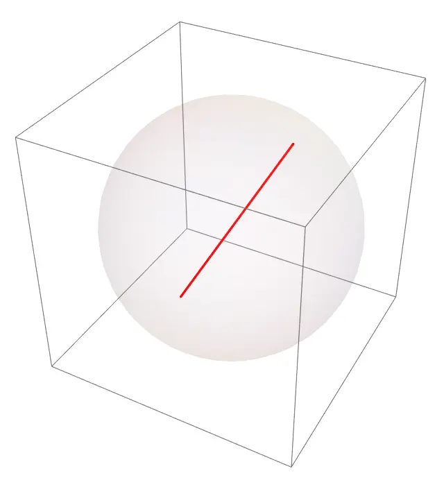
We find for this loop, the intersection number is not divisible by 4. Therefore, by the previous assertion, we conclude these loops are not homotopic to a constant loop, and hence form their own distinct class of loops. We will denote these as the non-trivial loops in $\rp^3$.

Glossing over technical details, it turns out, these are the only two classes of loops in $\rp^3$. Since loops two loops in different classes aren’t homotopic, we conclude they must belong to different path components of $\Omega \rp^3$. We will denote each path component as $\Omega^T \rp^3$ and $\Omega^N \rp^3$, which are the path components containing and not containing the constant loop.

As mentioned in theorem, $SF(S^2\times S^1)$ is homotopy equivalent to $\Omega \rp^3$, hence $SF(S^2\times S^1)$ contains two path components. We will denote $SF^T$ and $SF^N$ as path components of $SF(S^2\times S^1)$ containing and not containing the identity. In particular, each path component is homotopy equivalent to a path component in $\Omega \rp^3$, and since each path component in $\Omega \rp^3$ is homotopy equivalent to $\Omega S^3$, we arrive at the following relation: \(SF^T \simeq_H \Omega S^3, \jand SF^N \simeq_H \Omega S^3.\)

The immediate result of this observation is that $H_n(SF^N)$ and $H_n(SF^T)$ are the infinite cyclic group when $n$ is even, hence they are generated by one element. In the remainder of this article, we will focus on when $n=2$ and try to interpret these results from a more visual approach.Now here, one starts to wonder why we care about visualizing homology generators? One immediate application of understanding homology generators is its use in understanding induced maps between homology groups. In particular, understanding the maps of homology groups induced from maps between spaces can tell us a lot about the relationship of these spaces. To characterize these maps it suffices to only consider the action of the map on the generators. For this reason, having a visual understanding of these generators provides mathematicians with a more visual way to make these computations. For a more analytical analysis, I will refer you to [WY24, Section IV].

The Animations

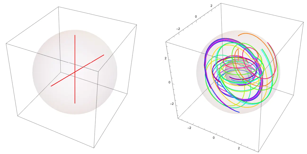
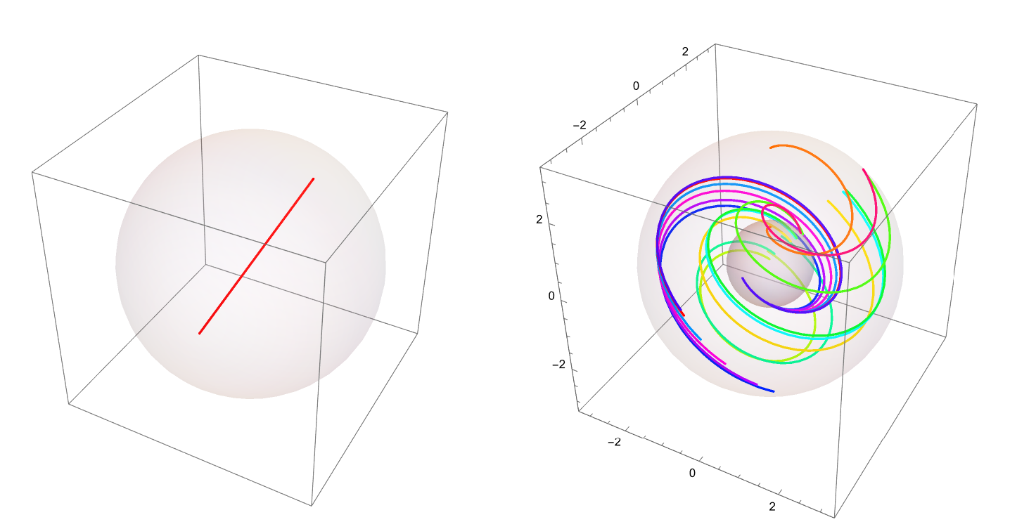
Now, we have finally reached the section where we can talk about the animations. To actually realize loops in $\rp^3$ in $S^2\times S^1$, we need to discuss how to map a loop in $\rp^3$ to a Seifert fibering. From before, we note that $\rp^3$ can be mapped to $\sym{SO}(3)$ by taking the ray to the origin as the axis of rotation and the distance from the origin as the magnitude of rotation. In particular, this map is a diffeomorphism, hence it induces an isomorphism on homology. Since $SO(3)$ has a natural action on $S^2$, we can use this to define a map from a loop in $SO(3)$ to $SF(S^2\times S^1, T)$. Namely, we can define the map \(\phi: \Omega SO(3) \to SF(S^2 \times S^1, T), \quad M_t \mapsto \psi_{M_t}\) and \(\psi_{M_t}: S^2 \times S^1 \to S^2 \times S^1, \quad (v,s) \to (M_s v, s).\) Hence, in the image below, the loop on the left in $\rp^3$ induces a diffeomorphism that transforms the trivial fibering to the fibering as shown on the right.

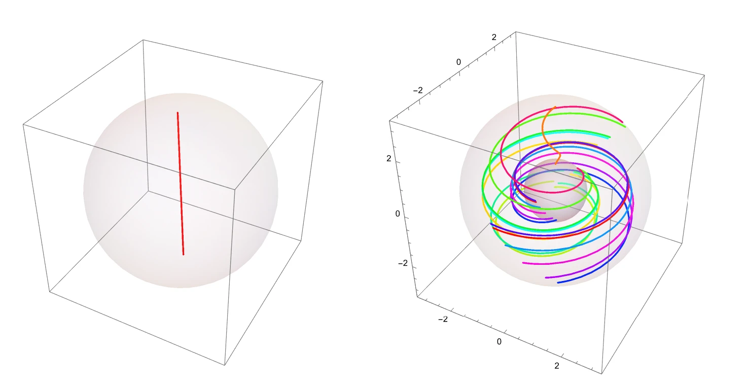
This map, in particular, is a homotopy equivalence, hence it induces an isomorphism on homology. In this way, we have simplified the problem of finding generators of $SF(S^2\times S^1,T)$ to a problem of finding the homology generators of $\Omega \rp^3$. I won’t go into the details of this calculation: more details can be found in [WY24]. As discussed before, $\Omega\rp^3$ has two path-components, each having a single homologous generator. For manifolds that we can easily visualize, a homologous generator is some type of generalized loop, but since our space here is in some sense infinite-dimensional (clearly by the fact that the homology of this space isn’t bounded), what a loop is in general might not be easy to see. But one thing we can be sure of is that we can understand each generator more easily by considering its image sets in $\sym{SF}(S^2\times S^1, T)$.

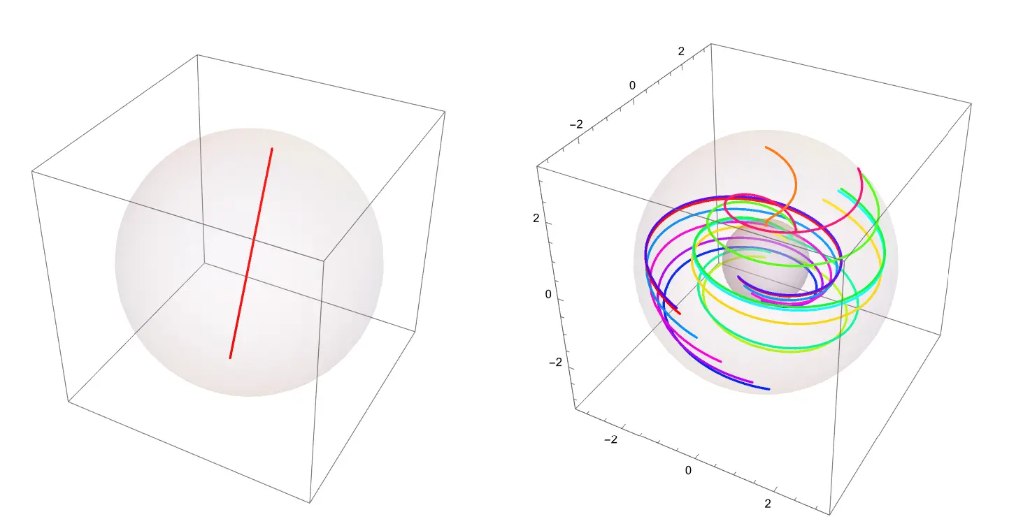
For $\Omega\rp^3$, we have the following generators: In the non-trivial component, we have the set of all loops that go through the sphere as in the image below

In the trivial component, we have the set of loops that are a composition of loops as described above. Below, we’ve included an example of a loop generated in the manner above.

Using the maps as described in this section, we can map these elements in the generators to $S^2 \times S^1$, and thus we get the following images:

For fun, we’ve also created the following animations for the viewers to ponder.

References

[WY24] Yi Wang, Jingye Yang. On the homotopy type of the space of fiberings of $S^2\times S^1$ by simple closed curves. arXiv preprint, arXiv:2404.08545, (2024).